No copy-editing has occured to provide this post some clarity. APA is almost ignored. But, the general curiosity remains. I have always been interested in identity and how we define ourselves throughout our lives and careers. The following was a brief paper and pilot “study” completed with a group of principals in 2006.

Very Brief Background

Q-factor analysis originated soon after Charles Spearman invented factor analysis at the start of the twentieth-century. Factor analysis, according to Steven R. Brown (1980), has been historically “used as a procedure for studying traits”. In this role, factor analysis has been popularized by social and political science. However, Brown explains that factor analysis can be used to factor persons, thereby creating what William Stephenson (1953) terms “person-prototypes”. This, Brown asserts, would require a separate methodology. This methodology, entitled Q, is described by Hair (1998) as “a method of combining or condensing large numbers of people into distinctly different groups within a larger population.”

Although G.H. Thompson was the first researcher to work with Q-factor analysis, he was not positive about its future (Brown, 1980). He believed that it had serious deficiencies, which I will discuss further in a moment. However, one researcher named William Stephenson was more excited about the possibilities of Q. Since its discovery, Q-factor analysis has been used widely in the social and behavioral sciences.

The main structural difference between Q and R analysis is summed up by Raymond Cattell’s description of the “data box” (1988). Cattell names three main components of a factor analysis: persons or cases, items, and occasions. He said that how we organize these components would structurally change the procedure. For example, in R-factor analysis the items signify columns on a matrix, while the persons completing the items represent rows. In this picture, one can see that the items would be grouped to create less factors, thereby creating types of items. Inversely, in Q-factor analysis, one can place the persons in the columns and the items in the rows. This process would create person-prototypes as previously mentioned.

The person-prototype idea is one that has revolutionized the social sciences. Researchers are able to make a case for a certain person type linked to various areas of behavioral disorders. One such study, conducted by Porcerelli, Cogan and Hibbard (2004), was created to better understand what personality traits men possessed who were violent towards their partners. The Q-sort was very large, 200 items long, and was completed by several psychologists and social workers very familiar with the many cases of domestic abuse. The end result supported the notion that these men were “antisocial and emotionally dysregulated.” Thus, it may be argued that these violent men have some things in common that make them stand out from others, person-prototypes.

Q-methodology has been employed by other fields of inquiry recently, as well. In Woosley, Hyman and Graunke’s work with student affairs problems on college campuses using a population of only three, the researchers wanted to explore whether Q would be a promising evaluation tool for the student experience (2004). They found, when asking these participants to sort ideas concerning their jobs on campus, that the students were excited about the process. During a post-sort interview, they all expressed enthusiasm for the activity and the results.

Controversy

Even with positive stories of Q like these, there are a few reasons why some researchers refuse to use this methodology or see any potential for its use. For example, one could easily discern from the discussion of the data box that a researcher could just take a set of data gathered for an R-factor analysis and apply it to the Q-structure, thereby completing another full analysis of the same information. Cyril Burt championed this form of usage in the Thirties (Stephenson, 1953). This is one point of contention for Stephenson. Stephenson explained that the procedure for collecting the data was part of the methodology. He stated that the Q-sort, the activity of participants physically sorting items in a prescribed pattern under certain conditions, was part of the overall methodology. One could not collect the data for the specific purpose of running an R-factor analysis and simply rearrange the data in a way appropriate for Q-analysis.

Many researchers disregard Q-factor analysis due to its lack of generalizability. They may claim that such a small sample could never be applied to a much larger population. In this respect, they may be correct. A Q-analysis is meant to really be something like a case study. It may be applied in some fashion to another situation, but the data collection is of a moment in time, or an occasion.

One of the main reservations I have with the Q-methodology is the focus on researcher-designated language. The language or items that are selected for the sort are done so by the researcher, not the participants. Thus, there may be some error in communication.

Sample Q-Sort Methodology

The particular focus of my sample Q-sort was a group of principals that are currently participating in the North East Florida Educational Consortium Principal Leadership Academy (PLA). The academy is only a year old, and the current version is a pilot run of the program that has been designed for principals who are undergoing some preliminary training to facilitate a school-wide action research project. The academy is comprised of twenty-four participants, principals with little experience or early-career principals to principals with a great deal of experience or seated principals. Because the leadership experience was quite varied among the group members, my hypothesis was these principals could be arranged in groups by experience and/or leadership style.

The items I decided to use in the Q-sort were the behaviors that the state recommended to the districts might be associated with the ten newly-adopted Florida Principal Leadership Standards (April, 2005). Of course, these behaviors were all optimal based on the standards. Thus, if a sort was using these written behaviors, there would be no “wrong” answers. This was important in establishing trust amongst the participants and me. This was no competition or evaluation of how they relate to and sort these behaviors. If they were aware at the outset, that there was no “correct” way to sort these items and there was no evaluative component to the sort, they may be more honest in the sorting process.

Another possible dimension that could be added to the sort that would possibly yield richer results would be the grouping of leadership behaviors into two categories, transactional leadership behaviors and transformational leadership behaviors. Due to the fact that these behaviors were never verified to actually represent either form of leadership, the Q-sort would have to be labeled an unstructured sort. (Appendix A).

After deciding which behaviors I would use as my items (16 sentence strips), I turned my attention to the actual Q-sort process.

Consulting Fred Kerlinger’s Foundations of Behavioral Research (1973), I was able to formulate a methodological plan. Kerlinger clearly maps out the process of setting up a practice Q-sort activity, or what he calls a “miniature Q-sort”. He writes that the participants may only sort a few items, as little as ten. This would not be optimal, he goes on to explain. Kerlinger insists the more items that one has available for the participants to sort, the better the results. Another piece of useful information was the discussion of the sort design. Kerlinger describes the physical act of sorting the items. He sets up a wonderful method of manipulating the items into a quasi-normal distribution, a Likert-type scale (with seven points) where the participant may choose whether the item is most like them or least like them. The participants are limited with the amount of items they can place at a given point. With this method of distribution, the sort resembles a normal curve. I used this example to help plan the sort activity with the principals in the PLA.

With the example below, the top line is the number of items that may be placed at each point on the Likert-type scale, and the bottom line is the scale itself. In this example, 7= items most like me, and 1= items least like me.

1 2 3 4 3 2 1
_________________

7 6 5 4 3 2 1

The sixteen items could be sorted in this quasi-distribution very easily by the participants. Each behavior strip contained a number, so that the participants could easily record the placement on the data sheet provided (Appendix B). I created ten identical envelopes containing the sixteen principal behavior strips. Then, I created a large poster displaying the procedures of the sort and the limitations for each placement. I would let the principals sort the behaviors after an already scheduled PLA meeting. They would be separated, mostly for the purpose of providing space for each participant.
On November 2, 2005, the participants completed the sort and carefully filled out the corresponding data sheet as I monitored. The purpose for monitoring was the successful completion of the stated procedures. This was explained to the participants. Once I collected all of the data, I began entering into SPSS 13 to start the analysis. The SPSS software is really set up with R factor analysis in mind, the columns are used for mostly organizing items (refer back to the discussion of Cattell’s idea of the Data Box). However, it is important to note that one may enter the participants in the columns as nominal data. Then, one could easily enter the numbers of the sorted behaviors as the rows. Then, the factor analysis procedure is the same from this point on.

Analysis and Interpretation

In this discussion of the results of this particular practice Q-analysis, I will be addressing the interpretation of the results yielded in Q-analysis in general. I will also be referring to Figures 1-7, yielded by the SPSS software during this practice analysis.

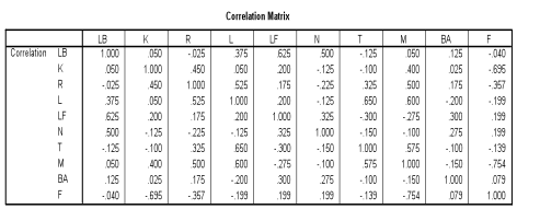
Figure 1 displays the correlations between the individuals based on how they sorted the leadership behaviors. We started with ten factors (individuals), and we are given ten separate factors in this table. This matrix enables the researcher to make some general statements about how each participant correlated with another. Remember, a 1.0 is a perfect correlation, so those are usually the person correlated with themselves. If one consults Hair’s opinion on the cut-off point for correlations, the cut-off for looking at correlations is anything under .450. This makes sense, because the researcher is really looking for correlations that are nearer to 1.0, as stated above. For example, one can see that there exists a strong correlation between LF and LB (.625). Thus, we could state that they may have sorted somewhat similarly. Inversely, M is not correlated to LB very well at all (.050), leaving us to assume that these two individuals may have sorted the behaviors very differently. However, this is all that we can ascertain at this point.

Table 1.

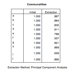
In Figure 2, the researcher is focused on communalities, or how much of the original participant/factor was extracted/recreated in the analysis. The glaring observation that should be seen at the fore is N (.557) shows the least in common with the group as a whole. At this point, it would help the reader to know that N was the only non-principal participant in the sort. I offered her the chance to take part in the sort to have an even number of ten participants in the activity. N has never worked in an educational administration position.

Table 2.

Extraction Method: Principal Component Analysis.

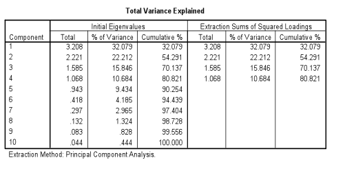
The next step in the analysis is to look at the Eigenvalues and percent of variance that may be explained by the factor analysis (Table 3). When the data was entered, I wanted to isolate the factors that had Eigenvalues of 1.0 or greater. This would present four factors or, in the case of the SPSS output, components. These factors/components are the “person proto-types” discussed earlier. With this table, one can discern that almost 81% of the variance is explained in the analysis. This is very positive for two reasons: first, I now can see that four factors or person proto-types was a good number to represent most of the variance and, secondly, the low number of four factors is a good reduction from the original ten.

Table 3.

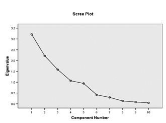
A scree plot of the factors will confirm that four factors/components is a good representation of the whole. To read the scree plot in Figure 1, one must look for the area at which the downward motion of the line comes to a plateau or a leveling off. It is apparent to me that the original interpretation of the number of factors was a wise decision. The plateau of the scree appears after the fourth factor. One may argue that this point actually does not level off as much as it jets upward slightly. However, being aware that this point represents the odd-man out, N (the participant with no experience in an educational leadership role), I believe that four factors truly does represent the whole in the best way. After reviewing this output originally, I ran the analysis again isolating only three factors. However, there ended up being a few of the original participants/factors left out of the whole. Thus, I opted for the four-factor analysis model.

Figure 1.

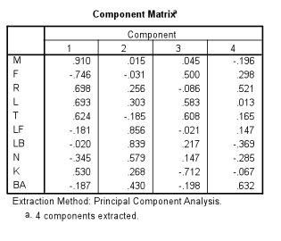
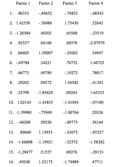
In the next step of the analysis, the researcher begins to examine the extent to which each original factor is represented by the four composite factors or proto-types. The first matrix (Table 4) shows the extent to which each of the original components is represented by the four factors created before the rotation and the variance is distributed more evenly amongst the factors. In other words, we can see which of the person-prototypes each individual fits in the best. For example, M is definitely more associated with the first extracted factor. With this matrix, we can only begin to see how the participants might relate to the person proto-types created. To gain a clearer picture of the relationship between the participants and the composite factors, one needs to consult the rotated component matrix.

Table 4.

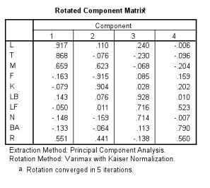
In Table 5, the output from the rotation (using the varimax criterion) is more accurate in describing how the well the components is represented by each of the factors. With the background knowledge of all the participants, I could easily see justification for each of the participant’s placement in the matrix. I set the analysis in SPSS to create an output that would arrange according to size. Thus, looking at the matrix, the researcher can see the participants that share the most in common grouped together. In the first column, the first three participants are strongly correlated at .917, .868, and .659 respectively. It is interesting to note that these three principals represented by the first factor are the three most experienced of the participants. Additionally, these three administrators started a statewide reading reform together, meeting monthly for the last five years to discuss and share ideas with reference to the reform.

Table 5.

In the next factor, F (-.915) and K (.904) are represented. F, it appears, is very negatively correlated to K. K has been a principal for one year and has worked as an assistant principal to one of the participants represented in the first factor. F was the principal of a failing school last year, and now is a new principal at a K-22 special needs school. They actually appear to have sorted the behavior strips almost the exact opposite of each other.

The third factor has LB (.928), LF (.716), and N (.714) correlated to each other. LB and LF are both first year principals. N is the non-principal among the group as stated previously. It makes sense to me that they may have sorted the behaviors similarly.

The final factor includes BA (.790) and R (.560). R does not appear to correlate highly with any of the four factors. This grouping is the only one that seems to contain two individuals that have very little in common in their backgrounds. When I forced the analysis to create only three factors/components, BA was left out of the final grouping of factors.

Before leaving the analysis, it is important to speak to one last piece, the variables/behavior strips and their value to each of the factors (Table 6). These values are in the form of Z-scores, making it easier to see how each person- prototype sorted each behavior (interpreted by columns) and how each behavior strip was comparatively sorted in each person- prototype (interpreting by rows). Daniel (1990) explains that these values or standardized regression factor scores are “utilized to determine which items contributed to the emergence of each of the person factors.” Remembering that the first eight strips were designated as transformational leadership behaviors and the second eight were designated as transactional leadership behaviors, one can now find some patterns in how the prototypes sorted. It could be argued that the first group organized the transformational leadership behaviors as more like them than the transactional leadership behaviors. For example, behavior strips # 1, 2, and 4 all score very highly in the matrix for the first group. In contrast, the third group scored behavior #1 negatively, less like them. However, the third group also scored transformational behavior strips # 2 and 4 highly.

Table 6.

Taking into account that the scores did not really follow a trend that established any of the groups as definitively transformational or transactional, it is probably safe to say that the participants were grouped according to another criterion. We can say that the participants were grouped with others who sorted a set of behaviors similarly on that day at that time.

There are two facets of the Q-sort and analysis that I would change if I were to conduct a similar study in the future. To begin, it would be more structurally sound to use many more behaviors in the sort. The added information that they could rate may yield different results in the analysis. Additionally, I would not group the Florida Principal Leadership Behaviors into the two leadership styles, transformational and transactional. This created an unstructured sort, or one based on items that were not used previously in this manner. There has been no research linking these particular items with the labels transformational and transactional.

This practice Q-sort and analysis is narrow in scope. Judgments concerning the principals’ sorts are not applicable. The purpose of this study was to simply find out if the principals could be placed into groups or factors that seemed to make sense. Knowing the backgrounds of the participants allowed me a different lens at which to look at the analysis that many researchers may not get when conducting a Q-sort. It allowed me to understand why I think the participants grouped the way they did.

Citations

Brown, S. R. (n.d.) The history and principals of q social sciences methodology in psychology and the social sciences. Retrieved Nov 2, 2005, from http://facstaff.uww.edu/cottlec/QArchive/B.

Brown, S.R. (1980). Political subjectivity: applications of q methodology in political science. London: Yale University Press.

Daniel, L. G. (1990). Operationalization of a frame of reference for studying
organizational culture in middle schools (Doctoral dissertation, University of New Orleans, 1989). Dissertation Abstracts International, 50, 2320A.
(UMI No. 9002883)

Hair, J., Tatham, R., Anderson, R., & Black, W. (1998). Multivariate data analysis. 5th ed. New York: Prentice Hall.

Kerlinger, F. (1973). Foundations of behavioral research. 2nd ed. New York: Holt, Rinehart and Winston, Inc.

Nesselroade, J., & Cattell, R. (1988). Handbook of multivariate experimental psychology. 2nd ed. New York: Plenum Press.

Porcerelli, J. H., Cogan, R., & Hibbard,S. (2004). Personality characteristics of partner violent men: a q-sort approach. Journal of Personality Disorders, 18(2), pg. 151-162.

Stephenson, W. (1953). The study of behavior. 2nd ed. Chicago: The University of Chicago Press.

Woosley, S. A., Hyman, R. E., & Graunke S. S. (2004). Q sort and student affairs: a viable partnership?. Journal of College Student Development, 45(2), p.231-242.